Getting Started

The following section walks you through the fxs workflow. First lets setup the xframe home directory by calling:

$ xframe --setup_home HOME_PATH

and substituting HOME_PATH with where ever you want xFrame to store files by default, if no value for HOME_PATH is given ~/.xframe will be used.

Short version of getting started

If you are willing to skip first step of extracting correlations from scattering patterns, the short version of this tutorial consists of executing the commands

$ xframe fxs simulate_ccd tutorial
$ xframe fxs extract tutorial
$ xframe fxs reconstruct tutorial
$ xframe fxs average tutorial

and looking at the data outputed to 'HOME_PATH/data/fxs/'.

xframe fxs simulate_ccd generates a cross-correlation dataset
xframe fxs extract extracts the single-particle rotational invariants.
xframe fxs reconstruct runs phase retrieval using the computed invariants
xframe fxs average averages a set of provided reconstructions

You want it all in one command? No problem!
xFrame supports command chaining so you can equivalently just call

$ xframe fxs simulate_ccd tutorial extract tutorial reconstruct tutorial average tutorial

Note if you are running these scripts on a machine with less than 4 physical cpu cores you will have to run

$ xframe fxs reconstruct tutorial

twice and change the settings for the average command at HOME_PATH/settings/projects/fxs/average/tutorial.yaml before the averaging command can be run sucessfully. In the settings file change the lines

reconstruction_files:
  - 3d_tutorial/{today}/run_0/data.h5

to

reconstruction_files:
  - 3d_tutorial/{today}/run_0/data.h5
  - 3d_tutorial/{today}/run_1/data.h5

After exectuing the above command the following files and folders should exist

HOME_PATH
├── projects
│   └── fxs 
└── settings
    └── projects
        └── fxs
            ├── average
            │   ├── default_0.01.yaml 
            │   └── tutorial.yaml
            ├── correlate
            │   ├── default_0.01.yaml
            │   └── tutorial.yaml
            ├── extract
            │   ├── default_0.01.yaml
            │   └── tutorial.yaml
            ├── reconstruct
            │   ├── default_0.01.yaml 
            │   └── tutorial.yaml
            └── simulate_ccd
                ├── default_0.01.yaml
                └── tutorial.yaml

The path HOME_PATH/projects/fxs is a symlink to the installation folder of the fxs toolkit, while HOME_PATH/settings/projects/fxs contains the default settings for each tool as well as a tutorials settings file.

xFrame command structure

You can see all available fxs commands by calling:

$ xframe fxs --help

The general command structure is as follows:

$ xframe fxs COMMAND SETTINGS_NAME

where SETTINGS_NAME is the file name of the settings file to be used, e.g.:

$ xframe fxs reconstruct tutorial

will execute the reconstruction command using the the settings file located at HOME_PATH/settings/projects/fxs/reconstruct/tutorial.yaml. See Settings for details on xFrame settings management.

1. Creating a cross-correlation dataset

There are two options to generate an initial cross-correlation dataset. In 1a the xframe fxs correlate command is used to generate the cross correlation function from a set of scattering patterns. This however requires the download of a 2GB dataset. In 1b we simulate cross-correlations from a given density distribution.

If you try xframe fxs on a Laptop with only two or four physical cpu cores the computation in 1a will take between 60 and 120 minutes. So if you only want to try xframe quickly simulating the cross-correlation dataset as in 1b is recomended.

You may also chain commands to perform several actions in a row, e.g.:

$ xframe fxs reconstruct tutorial average tutorial

will first execute the reconstruction command using its "tutorial" settings file followed by a call to the averaging routine using its "tutorial" settings file.

1a. From scattering Patterns (Download required)

Please download the files/folder

├── 3d_diffraction_patterns_pentagonal_cluster
└── 3d_pattern_list.txt

from https://syncandshare.xfel.eu/index.php/s/bDQsfAnk5TNQadr. 3d_pattern_list.txt simply contains the folder paths of individual diffraction patterns that should be used in the cross-correlation calculation, whereas 3d_diffraction_patterns_pentagonal_cluster is a folder contining the scattering patterns.

The command line tool for extracting cross-correlation functions from scattering patterns is

$ xframe fxs extract SETTINGS_NAME

Let's open the settings file at HOME_PATH/settings/projects/fxs/extract/tutorial.yaml which should contain the following:

structure_name: 'tutorial'

image_dimensions: [512,512]

n_processes: 32

max_n_patterns: 2000


compute: ['is_good','waxs_aver','ccf_q1q2']
pixel_size: 200.0                 #Detector pixel size in microns
sample_distance: 800.0            #Detector to sample distance in [mm]
wavelength: 1.23984               #X-ray wavelength in Å
detector_origin: [255.2,255.5]    #2D detector origin in pixel coordinates

interpolation_order: 2            #Cartesian to Polar spline interpolation order

phi_range:                        #Azimutal angle grid via (start,stop,npoints,???)
    command: '(0.0, 2*np.pi, 1024, "exact")'
fc_n_max: 70                      #maximal resolved harmonic order


IO:
  folders:
    home:
      command: 'xframe_opt.IO.folders.home'
    in_base:
      home: 'data/fxs/input_files/'
  files:
    input_file_list:
      name: patterns_list.txt
      folder: in_base

The IO: option at the end of the settings file tells xframe where to find or save files.

E.g. the above contents IO tell xframe to look for the input_file_list at HOME_FOLDER/data/fxs/input_files/patterns_list.txt. To change the location you can, just put the folder path which contains your downloaded file in the in_base option, i.e.:

in_base: PATH_TO_FOLDER_CONTAINING_THE_DOWNLOADED_FILES/

instead of

in_base:
  home: data/fxs/input_files/

To start the computation we can now call:

$ xframe fxs correlate tutorial

Once the computation is done continue in section Output.

1b. Simulating cross-correlation dataset from a given density (no Download required)

Executing the following command generates a cross-correlation dataset.

$ xframe fxs simulate_ccd tutorial

The creation of the cross-correlation data set should take about 1-2 minutes.

While the computation is runnig lets take a look at the sittings file which should look as follows.

dimensions: 3

structure_name: 'tutorial'

grid:
  max_q: 0.322416
  n_radial_points: 512
  max_order: 128

shapes:
  types:
    command: "['tetrahedron']*6"
  centers:
    command: "[(0,0,0)] + [(140.0,np.pi/2,phi*2*np.pi/5) for phi in range(5) ]"  #3D centers
    #command: "[(0,0)] + [(140.0,phi*2*np.pi/5) for phi in range(5) ]"           #2D centers
  sizes:
    command: '[70]*6'
  densities: [25,50,25,50,25,50]
  random_orientation:
    command: '[True]*6'
cross_correlation:
  method: 'back_substitution'
  xray_wavelength: 1.23984

The dimensions option speciefies wether to generate cross-corrleations from a 2D or a 3D density. Under grid one can set the basic parameters for the grid size.

max_q: Maximal momentum transfer value in Angstöm.
n_radial_points Number of radial grid points in both real and reciprocal space.
max_order Maximal considered harmonic order (determines the angular grid)

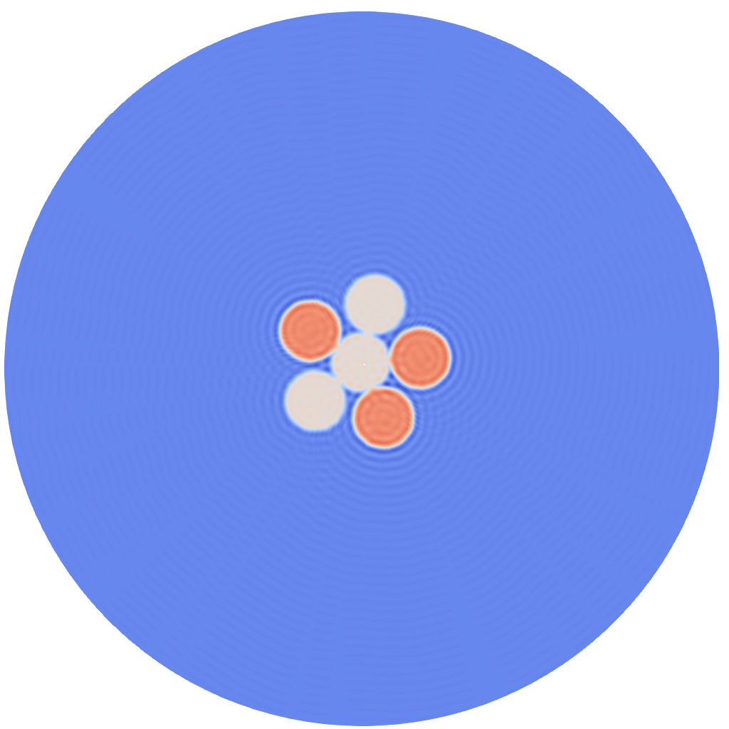
The shape option contains the description of the density to be used. In this case we generate 6 spheres with 70nm radius in a pentagonal pattern half of which have density 50 and the other half 25. Note that instead of specifying a settings value directly one can create a subentry called command:. Any string contained in this entry will be executed as python command and stored in the above settings entry.

Possible values for types are ('sphere','cube','tetrahedron'), if dimensions is set to 2 'cube' will result in a square and 'thetrahedron' in a regular triangle.

Under cross_correlation options are listed that specify which formula should be used to generate Cross-correlation function in the 3D case. Possible values for method are (back_substitution,lstsq,legendre). The unit of xray_wavelength is Angstöm, it is used to take the ewald's sphere curvature into account. For details on the used formulas see extract In the two dimensional case (dimensions: 2) these options have no effect.

Output

Upon completion of either section 1a or 1b the following files should have been generated.

HOME_PATH/data/fxs/
└── ccd
    ├── 3d_tutorial.h5                      #symlink to ccd.h5 from below
    └── archive
        └── 3d_tutorial
            └── DATE
                └── run_0
                    ├── settings.yaml
                    ├── ccd.h5
                    └── model_density.vts   #only for section 1b

Here settings.yaml contains the parsed settings file used in the computation. This settings file will additionally to the above shown options contain all default options which have not been changed. The main data output is the ccd.h5 file which contains the following fields:

ccd.h5
├── radial_points
├── angular_points
├── xray_wavelength
├── average_intensity
└── cross_correlation
    └── I1I1

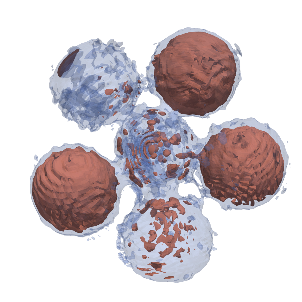
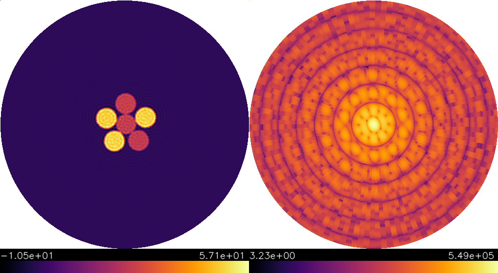
In case the cross-correlation was created from an electron density the corresponding model density is saved in model_density.vts, which can be visualized with paraview:

3D model (1b.)	2D model (1b.)

If more calls to either xframe fxs correlate tutorial or xframe fxs simulate_ccd tutorial are made the results will be saved to folders called run_1, run_2,… and the 3d_tutorial.h5 symlink will be updated to the latest calculation. This symlink points to the default dataset used in the following invariant extraction step. Automatic symlink updates to the newest calculation can be turned off by modifying the settings file under IO as follows:

IO:
  files:
    ccd:
      options:
        save_symlink: False

2. Extract invariants

This section is about using the cross-correlation data to extract the single-particle rotational invariants

\[
\begin{aligned} B_l(q_,q_2)=\sum_m I^l_m(q_1)I^l_m(q_2)^* && B_n(q_1,q_2)= I_n(q_1)I_n(q_2)^* \end{aligned}
\]

and their associated projection matrices $V^l_o(q),v_o(q)$ that satisfy

\[
\begin{aligned}
I^l_m(q)=\sum_{o} V^l_m(q) U^o_m && I_n(q)= v_n(q) u_n &&
\end{aligned}
\]

for unknown unitary matrices $U$ and $u$.

Here $B_l(q_1,q_2)$ are the invariants under three dimensional rotations with $I^l_m$ beeing the single particle spherical intensity harmonic coefficients, while $B_n(q_1,q_2)$ are invariant under two dimension rotations with $I_n$ denoting the intensity Fourier series coefficient.

Calling

$ xframe fxs extract tutorial

will compute these invariants depending on the chosen dimension settings (this computation sould take about 3 minutes).

Settings

The tutorial settings file contains the following options

dimensions: 3

structure_name: 'tutorial'

max_order: 69

extraction_mode: 'cross_correlation'

cross_correlation:
  datasets_to_process: ['I1I1']
  datasets:
    I1I1:
      bl_extraction_method: 'back_substitution'
      assume_zero_odd_orders: True
      modify_cc:
        subtract_average_intensity: True

IO:
  folders:
    base:
      command: 'xframe_opt.IO.folders.home'
    data:
      base: 'data/fxs/'
    ccd:
      data: 'ccd/'
  files:
    ccd:
      name: 3d_tutorial.h5
      folder: ccd

In the dimensions: 3 case there are three possible invariant extraction methods that can be specified in the bl_extraction_method: option.

The default option is back_substitution which solves the following equation using back substitution for the Invariants $B_l$:
```
\[
\begin{aligned}
C_n(q_1,q_2) &= \sum_{l\geq |n|} \overline{P}^{|n|}_l(q_1)\overline{P}^{|n|}_l(q_2) B_l(q_1,q_2)\\
\overline{P}^{|n|}_l(q)&= \sqrt{\frac{(l-n)!}{4\pi(l+n)!}} P^{|n|}_l(\cos(\theta(q)))
\end{aligned}
\]
```
where $C_n(q_1,q_2)$ denotes the $n'th$ circular harmonic coefficient of the cross correlation $C(q_1,q_2,\Delta)$, the $P^{|n|}_l$ are associated Legendre polynomials and $\theta(q)= \arccos(q/(2\lambda))$ describes the ewald's sphere curvature and depends on the laser wavelength $\lambda$.

If lstsq is selected the following relation is solved using a least squares solver:

\[
\begin{aligned}
C(q_1,q_2,\Delta) &= \sum_{l=0} F_l(q_1,q_2) B_l(q_1,q_2)\\ F_l(q_1,q_2)&= \frac{1}{4\pi} P_l(\cos(\theta(q_1))\cos(\theta(q_2))+\sin(\theta(q_1))\sin(\theta(q_2))\cos(\Delta))
\end{aligned}
\]

where $P_l(q)$ are ordinary Legendre polynomials.

Finally if legendre we use the flat Ewald's sphere (small scattering angle) approximation and solve:
```
\[
\begin{aligned}
C(q_1,q_2,\Delta) \approx \sum_{l=0}  \frac{1}{4\pi} P_l(\cos(\Delta)) B_l(q_1,q_2)
\end{aligned}
\]
```
by using an inverse Legendre transformation.

The settings entry max_order: allows one to choose the highes harmonic order for which invariants should be computed. In setting assume_zero_odd_orders: True we use that the single particle intensity $I$ is real and therfore $B_l,B_n=0$ for all odd orders $l,n$.

Output

After the extraction is done the following files should have been created:

HOME_PATH/data/projects/fxs/
└── invariants
    ├── 3d_tutorial.h5
    └── archive
        └── 3d_tutorial
            └── DATE
                └── run_0
                    ├── extraction_settings.yaml
                    ├── first_arg_of_I1I1_Bl.png
                    ├── first_I1I1_Bl.png
                    ├── first_I1I1_proj_matrices_to_Bl.png
                    ├── mask_of_I1I1_Bl.png
                    └── proj_data.h5

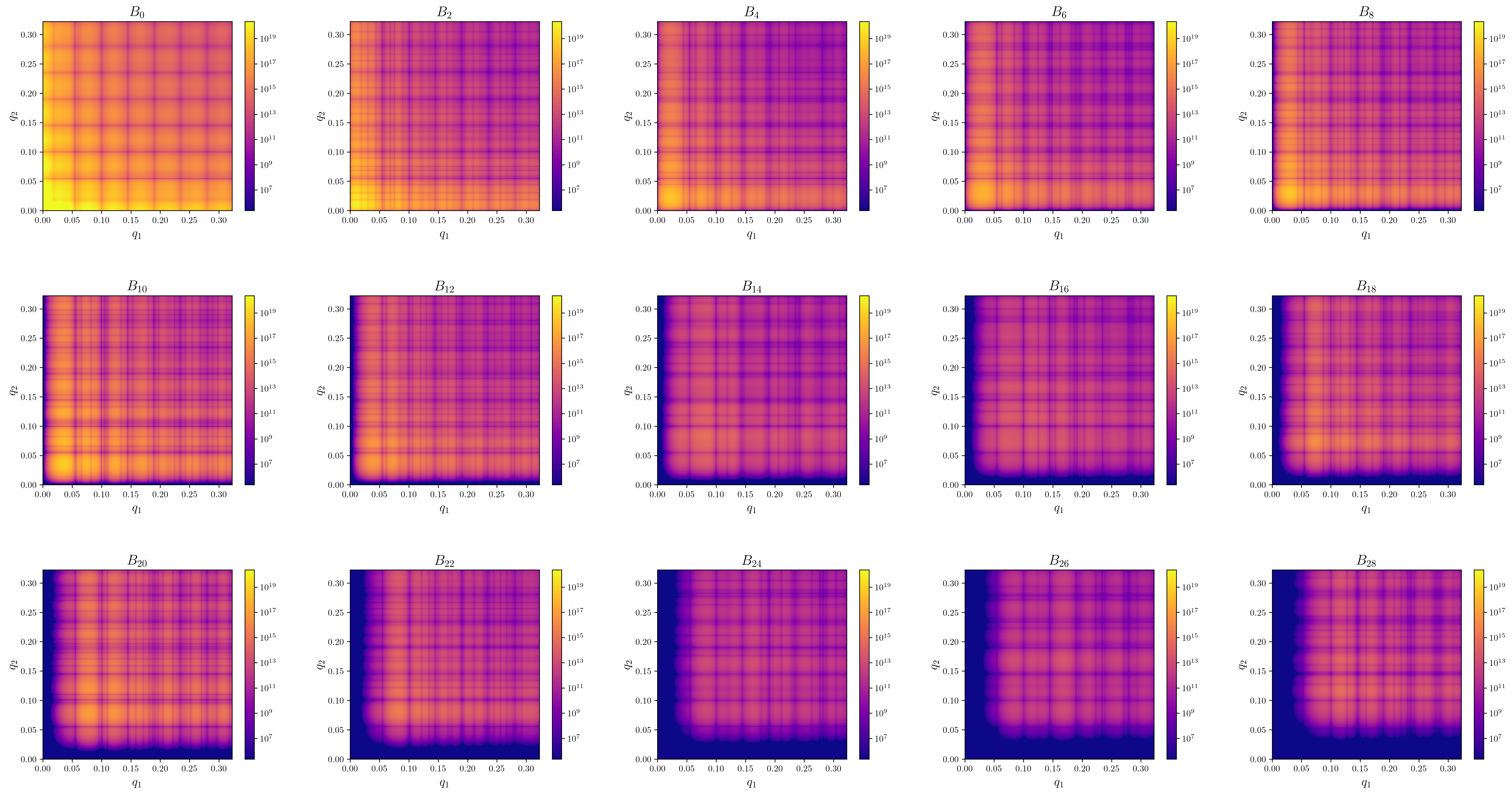
extraction_settings.yaml contains the parsed extraction settings including all default values.
first_I1I1_Bl.png Contains images of the absolute value of $B_l(q1,q2)$ for the first few orders.
first_arg_of_I1I1_Bl.png Contains images of the complex argiments of $B_l(q1,q2)$ for the first few orders.
first_I1I1_proj_matrices_to_Bl.png Contains images of $B_l(q1,q2)$ that where recalculated from the projection matrices via $B_l(q1,q2) = \sum_m V^l_m(q_1)V^l_m(q2)^*$. Since only the projection matrices are used in the reconstructon step, invariants calculated from reconstructions should be compared against these plots.

$B_l$ from patterns (3d 1a.) $B_l$ from density (3d 1b.) $B_n$ from density (2d 1b.)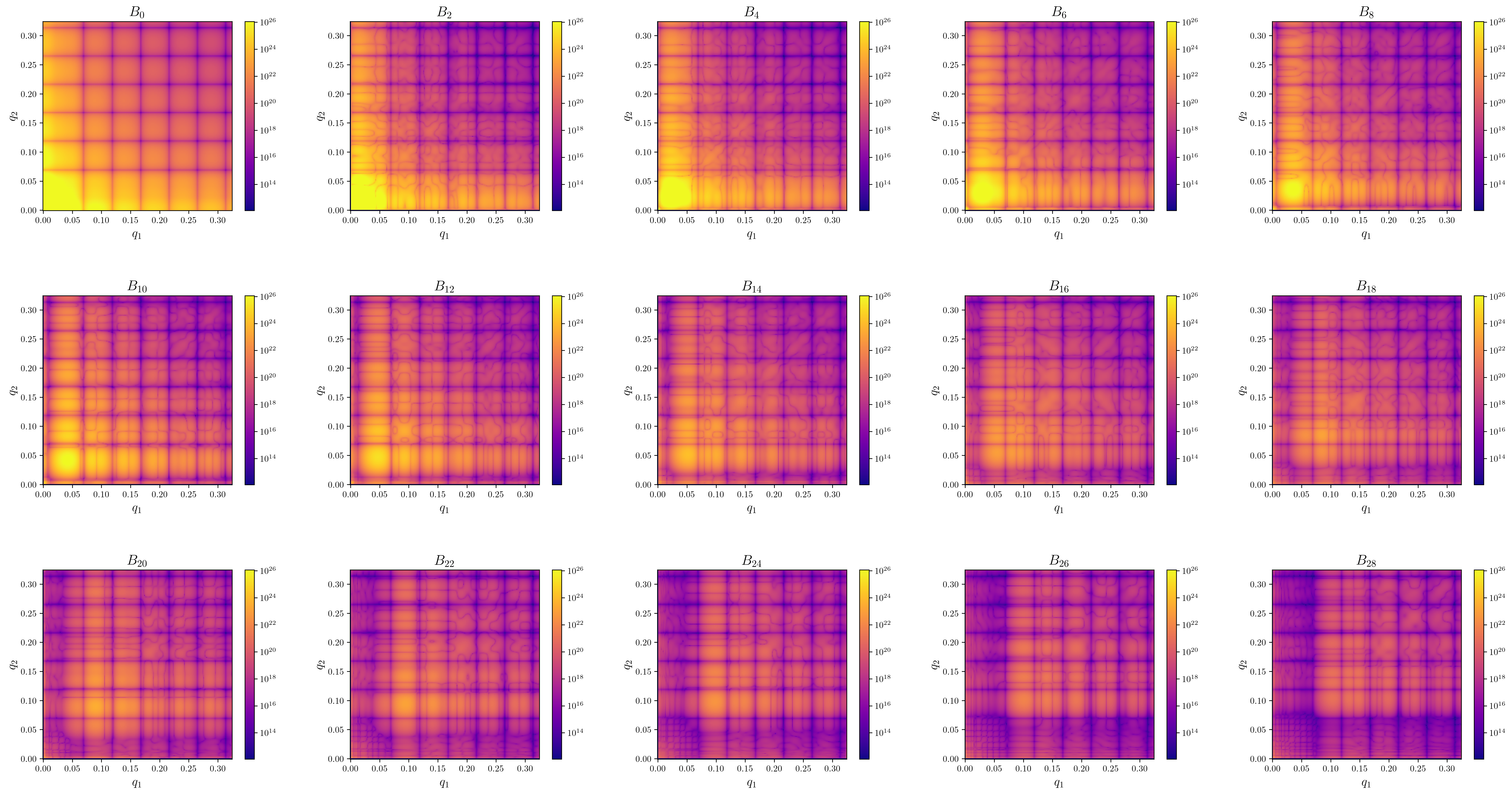
first_I1I1_Bl.png Contains images of the absolute value of $B_l(q1,q2)$ for the first few orders.
proj_data.h5 is the main data output file wich is used in the reconstruction step. It contains the following fields.

proj_data.h5 contents

├── dimensions
├── xray_wavelength                        # In Angstrom
├── max_order                              # Maximum harmonic order for which invariants where extracted
├── average_intensity                      # Angularly integrated average intensity <I>(q) (i.e.: SAXS)
├── data_angular_points                    # Angular grid points of cross-correlation
├── data_radial_points                     # Radial grid points of cross-correlation
├── data_projection_matrices
|   └── I1I1                               # V_l,v_n from our paper (I1I1 stands for I,I correlaitons) 
├── data_projection_matrices_q_id_limits
|   └── I1I1                               # Tuples of (q_min,q_max) for each harmonic order. ()
├── deg_2_invariant
|   └── I1I1
├── deg_2_invariant_q_id_limits
|   └── I1I1
└── deg_2_invariant_masks
    └── I1I1

3. Reconstruct

We can now use the extracted invariants to reconstruct the single-particle electron density by calling

$ xframe fxs reconstruct tutorial

Info

This step benefits grately from GPU usage, therfore we recommend to install opencl on your system! That is also true if you just try to execute the tutorial on your laptop with built in graphics.

the reconstruction algorithm automatically detects how many CPU cores your system has and starts as many reconstructoins in parallel as possible. Upon execution you should see the following mesage in your console:

$ xframe fxs reconstruct tutorial
Starting <N> processes.
Starting <N> processes.

 ------- Start <xframe.projects.fxs.reconstruct.ProjectWorker object at 0x7f8f0ae7fd10> ------- 

Spawning phasing processes executing:
Loops:
        main:            5x( 60xHIO 1xSW 40xER )
        refinement:      1x( 1xSW 100xER )

Starting <N> processes.

Computation time:

The reconstruction should take on the order of 10-30 minutes to complete, here are some runtimes:

Runtime	Parallel reconstructions	CPU	GPU
12 mins	57	AMD EPYC 7543	2x NVIDIA RTX A6000
21 mins	1	intel i5-7200U	1x intel HD620

Output during phasing:

During phase retrieval each individual process will print error metric updates to the console, here is an example

P1: main Loop:5 Method:HIO Last Errors: 
{'real_l2_projection_diff': 0.0001540794008058123, 'main': 0.0001540794008058123}  Best Error: 3.6420631562418133e-05
number of particles = [1], max_density=(124.16959859463208-0.2816136730610012j)

P1 stands for Process 1
main Loop:5 Method:HIO tells you that you are looking at data from the HIO step in the 5'th iteration of the reconstruction step called main.
In {'real_l2_projection_diff': 0.0001540794008058123, 'main': 0.0001540794008058123} all computed error metric values are displayed. In this case only the real_l2_projection_diff is comuted and directly used as the main error metric for the reconstruction.
Best Error: 3.6420631562418133e-05 informs you about the lowest recorded error value during the entire reconstruction running in this process.
number of particles = [1] lists the assumed number of particles for the reconstruction.
max_density=(124.16959859463208-0.2816136730610012j) corresponds to the current density value with maximal real part.

Settings

While the reconstruction is running lets have a look at the settings file, which should contain the following lines

structure_name: 'tutorial'
dimensions: 3
particle_radius: 250

grid:
  n_radial_grid_points: 128
  max_order: 63

density_guess:
  type: 'bump' #'bump','ball'
  bump:
    slope: 0.3 #rho(r) = e^(-slope*r_max^2/(r_max^2-r^2))
  amplitude_function: random
  random:
    SNR: 2

projections:
  real:
    shrink_wrap:
      sigmas: [[20,[False,5],-2],False]
      thresholds: [0.09,0.09]
    HIO:
      beta:
        command: '[[0.5,0.4,-1/250,500],[0.01,0.002,-1/200,200]]'
    projections:
      apply: [support,value_threshold,limit_imag]
      support:
        initial_support:
          type: 'max_radius'
        enforce_initial_support:
          apply: True
          if_error_bigger_than: 6e-3
      value_threshold:
        threshold: [0,False]
      limit_imag:
        threshold: 2

  reciprocal:
    number_of_particles:
      initial: 1
    use_averaged_intensity: True
    q_mask:
      type: 'none'
    used_order_ids:
      command: 'np.arange(64)'

multi_process:
  n_parallel_reconstructions: True
GPU:
  use: True

main_loop:
  sub_loops:
    order: ['main','refinement']
    main:
      methods:
        HIO:
          iterations: 60
        ER:
          iterations: 40
        SW:
          iterations: 1
      iterations: 5
      order: ['HIO','SW','ER']
    refinement:
      methods:
        ER:
          iterations: 100
        SW:
          iterations: 1
      iterations: 1
      order: ['SW','ER']

`main_loop`

Let's first take a look at the main_loop: option which specifies the phasing loop structure as well as the used error metrics. In this tutorial well focus on the loop structure and let the error specification be handled by the defaults file, for more details see reconstruct. Any sub entry under sub_loops that is not called order is considered to descibe a phasing block and the order:entry simply specifies the execution order of the given phasing blocks.
Each block must have the following entries:

mehtods: wich contains phasing loop types to be used in this block. Possible loop types currently are ER,HIO and SW. Each of these looptypes must have sub setting called iterations: which specifies the number or repeats of this loop type within the phasing block. The differnt types can have other settings specified, see reconstruct for details.
- ER represents the Error Reduction loop due to
- HIO represents the Hybrid Input-Output loop due to
- SW represents a Shrink Wrap step as proposed by
iterations: The numer of times this phasing block should be repeated
order: The order in which the specified loop types should be executed.

A custom phasing block may look as follows

custom:
  methods:
    HIO:
      iterations: 100
    ER:
      iterations: 5
    SW: 1
  iterations: 5
  order: ['HIO','ER','SW','ER']

which would create a block called 'custom' with execution order 5x( 100xHIO 5xER 1xSW 5xER ).

`projections`

This option contains all settings regarding operations that change the density during the phasing loop in real and reciprocal space. Consequently it contains the suboptions real: and reciprocal:. The specified options under real: are

shrink_wrap: Wich allows the specification of the shrinkwrap parameters used in each phasing block.
- sigmas: specifies the gaussian $\sigma$, in Å, to be used. Its value is a list whos $n$'s element specifies the $\sigma$ value in the $n$'s phasing block. Each entry in this list can either be a number, False or a linear ramp specifier.
  If False is specified the the half period resolution of the current grid is used, that is $\sigma=\pi \frac{N_q}{q_{\text{max}}}$, where $N_q$ is the number of radial grid points and $q_{\text{max}}$ is the maximal momentum transfer value. (The $\pi$ factor is due to the [$2\pi/Å$] unit for the radial coordinate in reciprocal space. For more information on the used grids see Grids).
Linear Ramp specifier:

A linear ramp can be specified as a list of the form

[start_value,[stop_value,stop_argument],slope]

This will set the sigma value for the $n_\text{SW}$'th call to the shrink-wrap type SW via:
```
\[
\sigma(n_\text{SW})=A*n_\text{SW} + B
\]
```
where $A$ and $B$ are chosen such that $\sigma(0)=$start_value. If slope is specified i.e. is not False $A=$slope. stop_value acts as a value boundary which when it is reached fixes $\sigma$ to its value for all subsequent calls. Finally if slope is uspesified but stop_argument is given the parameter $A$ is chosen such thatn $\sigma($stop_argument$)=$stop_value. The stop_value itself can also be specified as False in which case again the half period resolution is used.
- thresholds: Is a list containing a number for each phasing block. Each number specifies the cutoff density value in % relative to the maximal real part of the current density guess during a shrink-wrap call.
HIO: Contains options for the input output mapping of the HIO loop type.
- betas: regulates the negative feedback strength after each HIO execution. Its value is a list specifying the $\beta$ parameters for each phasing block. Each entry can either be a number or a list specifying a exponential ramp.
Exponential Ramp specifier:

which is structured as follows (this whole linear/exponential ramp is a bit of a mess and needs to be cleaned up in future releases, sorry for that …).

[start_value,stop_value,exponent,stop_argument]

the $\beta$ value will be calculated for each execution of the HIO step via:

$$ beta(n) = Ae^{n*text{exponent}}+B $$
with $A$ and $B$ chosen such that $\beta{0}=$start_value and $\beta($stop_argument$)=$stop_value. One caveat here
projections: Contains all options regarding the realspace constraint.
- apply: A list containing the names of all constraints to be applied. (The constraints are applied in the order specified by this list.). The options for each specified constraint are stored in a sub option of projections: with the same name. Currently the following constraints are supported limit_imag,value_threshold and support.
- support: Spcifies the support constraint.
  - initial_support: Options for creating the initial support mask
    - type: only current value is 'max_radius'.
    - max_radius: If specified its value defines the radius of the spherical support mask in units of [Angstrom] other if not given the value specified in the gneral option particle_radius: is used.
  - enforce_initial_support: Specifies when to limit updates of the support mask to be contained in the initial support. Empirically we found that this helps with initial convergence.
    - apply: values are False or True.
    - if_error_bigger_than: If this option is present and contains a float. The support updates are only constraint to the initial support volume if the error metric is higher than the specified float. This option lessens Gibbs phenomenon artefacts (ringing) cauesed by reconstrucitons beeing to close to the initial support boundary.
- value_threshold: Limits the values the real part of the electron density can take.
  - threshold A list of 2 numbers [lower_limit,upper_limit], if falls is provided for either limit it is set to $\pm \infty$. Real part density values outside of this range are projected to the corresponding boundary value. This can for example be used to enforce positivity of the electron density by setting threshold: [0,False].
- limit_imag: Enforces a boundary on the imaginary part of the electron density.
  - threshold contains a positive number. Any imaginary density value whose absolute value is bigger than this number is projected to 0.

The specified options under reciprocal: have the following purpose:

use_averaged_intensity: True|False, if True the averaged intensity (SAXS profile) is used to define the zero'th order projection matrices $V_0$(3D) or $v_0$(2D).
number_of_particles:Contains options concerning the assumed average number of particles per scattering pattern that where used to generate the invariants $B_l,B_n$ and susequently the projection matrices $V_l,v_n$. Currently it is only possible to specify a fixed initial value.
- initial:Contains a number $N$. This will divide the given zeroth order projection matrix by $\sqrt{N}$.
q_mask: Allows to specify momentum transfer limits for the application of the reciprocal space constraints. The above given value 'none' assumes no limits, for details on more options see reconstruction
used_order_ids: Allows users to specify a list of harmonic orders on which the reciprocal constraint is enforced.

`density_guess`

This part of the settings file concerns the initial density guess with which a recnostruction is started. Current supported types are ball and bump. ball uses as envelope function a ball whose radius $r_\text{max}$ is given by the global option particle_radius. bump corresponds to the envelope function beeing a bump/test function given by $\rho(r)=e^{-s*r_\text{max}^2/(r_\text{max}^2-r^2)}$. For $r>r_\text{max}$ the functions value is set to 0. Its smooth drop off to 0 causes less ringing due to the gibbs pheneomenon at during the inital steps of the phase retrieval. The final density is obtained by multiplying the envelope function with random numbers generated by an amplitude function.

type: 'ball' or 'bump'
slope only used for type bump. Specifies the constant 's' in the expenent of the test function. Lower values cause a sharper drop off at the radial boundary set by $r_\text{max}$.
amplitude_function: Controlls the random number distribution inside the density guess currently it can only have the value 'random'.
- SNR: Allows to set the signal to noise ratio for the random number generator.

Output

After the reconstruction process is finished the following files should have been created.

HOME_PATH/data/fxs/reconstructions/
└── 3d_tutorial
    └── DATE
        └── run_0
            ├── RECONSTRUCTION_NUMBER_out_Bl.png
            ├── data.h5
            ├── error_metrics.png
            ├── first_Bl.png
            ├── settings.yaml
            ├── pics (only in the 2d case)
            |   └── reconstruction_RECONSTRUCTION_NUMBER.png
            └── vtk
                ├── real_RECONSTRUCTION_NUMBER.vts
                └── reciprocal_RECONSTRUCTION_NUMBER.vts

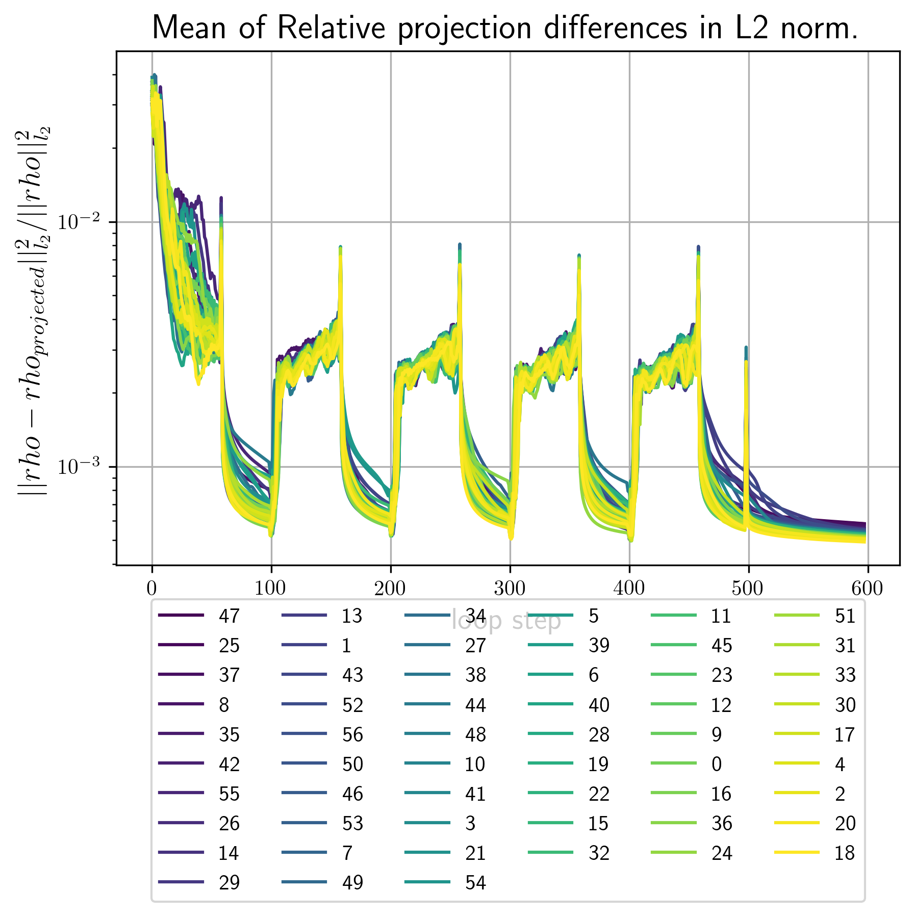
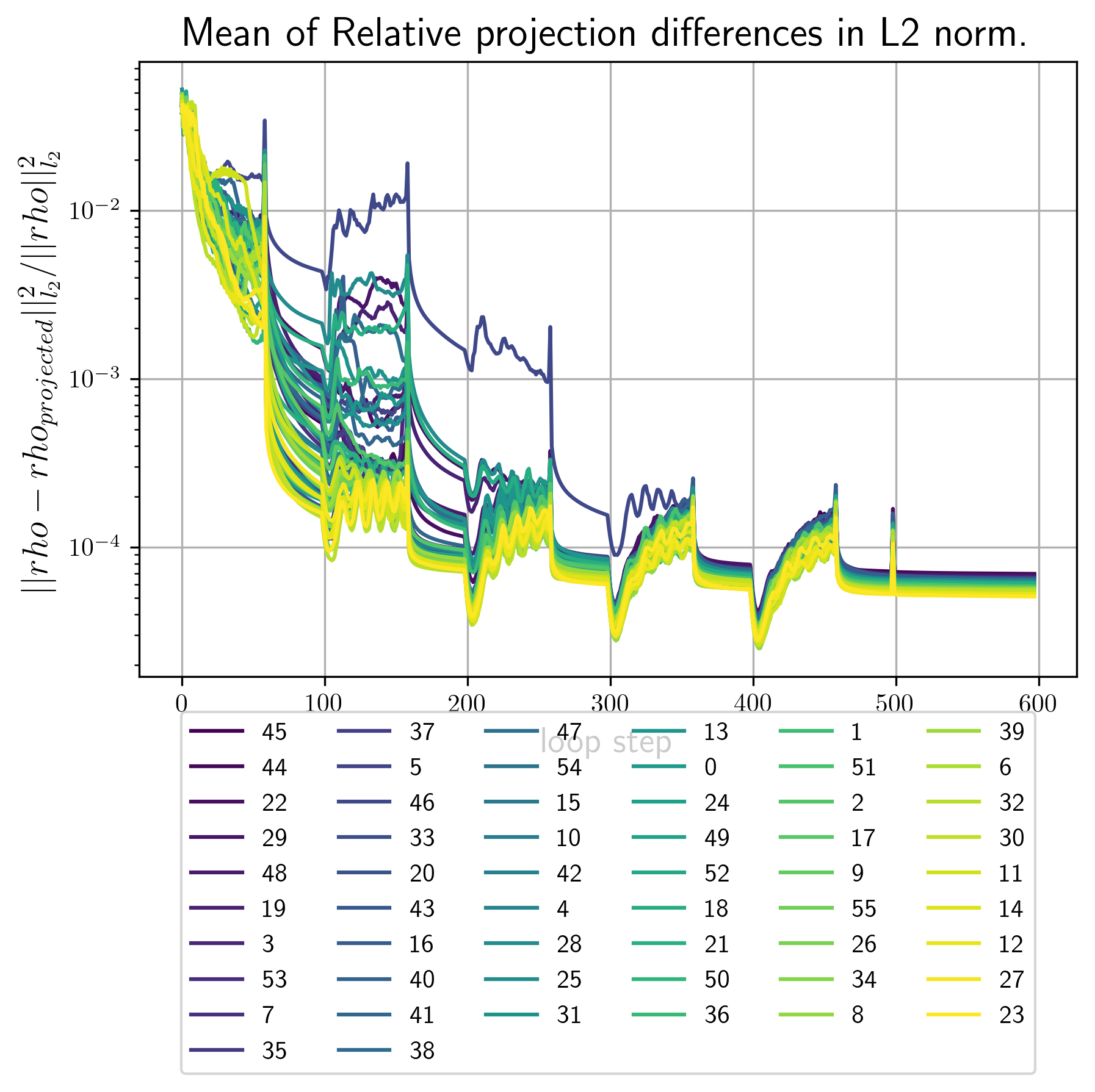
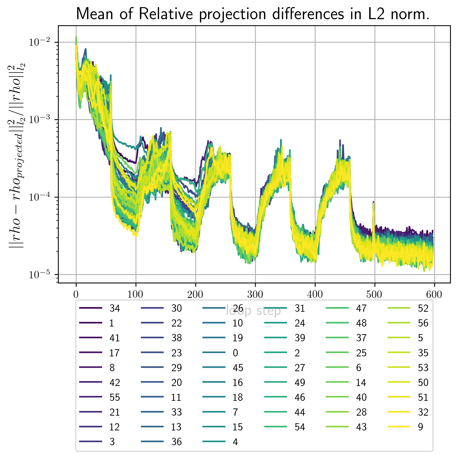
- settings.yaml Used settings including options set to their default value. - error_metrics.png Plots of the main error metric values for all reconstrctions. Here is an example

Example image

3d 1a.	3d 1b	2d 1b

first_Bl.png Contains images of the first few invariants that where used as input for this reconstruction run.
<RECONSTRUCTION_NUMBER>_out_Bl.png contain images of the $B_l,B_n$ invariants calculated from the final density. The better these images conincide with the ones in fisrt_Bl.png the better the convergence rate of the reciprocal constraint.
vtk Folder that contains vtk datasets. By default vtk files are generated for the best 2 and the worst reconstruction by error metric.
real_<RECONSTRUCTION_NUMBER>.vts vtk file for the electron density
real_<RECONSTRUCTION_NUMBER>.vts vtk file for the intensity. Single reconstructions depending on the input files from 1. may look as follows

3d 1a.	3d 1b.	2d 1b.

pics only for 2d reconstructions. It contains .png images of all computed reconstructions.
data.h5 is the main putput file.

data.h5 structure

data.h5
├configuration
│ ├internal_grid
│ │ ├real_grid
│ │ └reciprocal_grid
│ ├reciprocity_coefficient
│ └xray_wavelength
├projection_matrices (1 attributes)
│ ├ 0
│ ┆
├reconstruction_results
│ ├ 0
│ │ ├error_dict
│ │ │ ├main
│ │ │ ├real
│ │ │ │ └l2_projection_diff
│ │ │ └reciprocal
│ │ ├final_error
│ │ ├fxs_unknowns
│ │ │ ├ 0
│ │ │ ┆
│ │ ├initial_density
│ │ ├initial_support
│ │ ├last_deg2_invariant
│ │ ├last_real_density
│ │ ├last_reciprocal_density
│ │ ├last_support_mask
│ │ ├real_density
│ │ ├reciprocal_density
│ │ ├support_mask
│ │ ├n_particles
│ │ └loop_iterations
| ┆
└stats
  └run_time

4. Align and average

Since we only used orientation and position invariant constraints in the reconstruction, all computed densities are shifted, point inverted and rotated with respect to each other. This means that in order to average over several reconstructions we first have to align them.

In the two dimensional case there is a way around the rotation problem, by using the overall rotational freedom, i.e. we can use one global rotation as additional constraint alongside the invariants $B_n$. That is why previousely computed 2d reconstructions should only differ by point-inversion and shifts. In the three-dimensional case this is not possible. Here we allign densities by selecting a reference reconstruction and comparing all other reconstructions to this reference. The same approach is used to correct for point inversion in the two-dimensional case.

The command for alignment and averaging is

$ xframe fxs average tutorial

If the system this tutorial is executed on has more than 4 physical cpu cores (i.e. more than 8 hyperthreads) you can go ahead and execute this command directly.

If not the previouse reconstruction command onle genreates a single reconstruction at a time and you will have to call it a second time to get at least two structures that can be averaged. In this case we also need to tell the averaging routine to use a second reconstruction data file by uncommenting (i.e. remove the #) in the line:

#- 3d_tutorial/{today}/run_1/data.

Settings

The tutorial settings are given by

structure_name: 'tutorial'

reconstruction_files:
  - 3d_tutorial/{today}/run_0/data.h5
  #- 3d_tutorial/{today}/run_1/data.h5
  #- 3d_tutorial/4_2_2042/run_0/data.h5

multi_process:
  use: True
  n_processes: 20

selection:
  error_metric: 'main'
  method: "least_error"      #"least_error" or "manual"
  error_limit:  0.01         #only reconstructions with lower erros will be used
  n_reconstructions: 100     # <number> or 'all'. Limits the used number of reconstructions

center_reconstructions: True
normalize_reconstructions:
  use: True
  mode: 'max'                # 'max' or 'mean'

find_rotation:
  r_limit_ids:               # List of radial shell ids to be used in rotational alignment
      command: 'np.arange(20,80,2)'

l2_error_limit: 0.5          # The relative difference between reference and aligned pattern is larger
                             # exclude the alinged pattern from the average.
                             # Typical values (good alignment <0.1) (bad alignment >0.5) 



resolution_metrics:
  PRTF: True

Under the reconstruction_files: option you can specify the reconstruction datasets to be used. The file paths are parsed relative to 'HOME_PATH/data/fxs/reconstructions/' moreover there is the posibility to use the {today} modifier. If today would be July 1'st, 2023 the specified path in the settings file would point to:

'HOME_PATH/data/fxs/reconstructions/3d_tutorial/1_7_2023/run_0/data.h5

selection: regulates which reconstructions are to be aligned and how the reference structure is selected.
- method: least_error or manual | Selects as reference the reconstruction with lowest errror metric value or the one specified in the manual sub option.
- manual_specifier: list of 2 integers [FILE_ID,RECONSTRUCITON_ID] | only used when method: is set to manual
- error_limit: number | Only aligns reconstructions with error metrics lower then the threshold specified here.
- n_reconstructions: int or 'all' | Use maximal this number or reconstructions.
center_reconstructions: True or False| Whether or not to center reconstructions to their center of density.
normalize_reconstructions: Normalization options.
- use: True or False| Whether to normalize or not.
- mode: 'max'or 'mean' | Normalize maximum or mean value to 1
find_rotation: rotational alignment options.
- r_limit_ids :list or numpy array | Containing ids of the spherical shells which should be used in the alignment process. This is to exclude shells which contain no information about the rotational state of your reconstruction, e.g areas autside of the support or areas of almost constant density values.
l2_error_limit: number | For eachaligned pattern its relative overlap with the reference structure is computed $\text{err}=\frac{||\rho-\rho_\text{ref}||_{L^2}}{||\rho_\text{ref}||_{L^2}}$ if this value is higher than the given limit exclude the particular reconstruction from the final average.

Output

The following output files should have been generated after a call to xframe fxs average

HOME_PATH/data/fxs/averages/
└── 3d_tutorial
    └── DATE
        └── run_0
            ├── settings.yaml   
            ├── average_results.h5
            ├── PRTF.png
            └── vtk         
                ├── real_average.vts    
                └── reciprocal_average.vts

settings.yaml Used settings file with included default options.
PRTF.png Phase tretrieval transfer function for the averaged structure. Here are some examples

3d 1a.	3d 1b.	2d 1b.

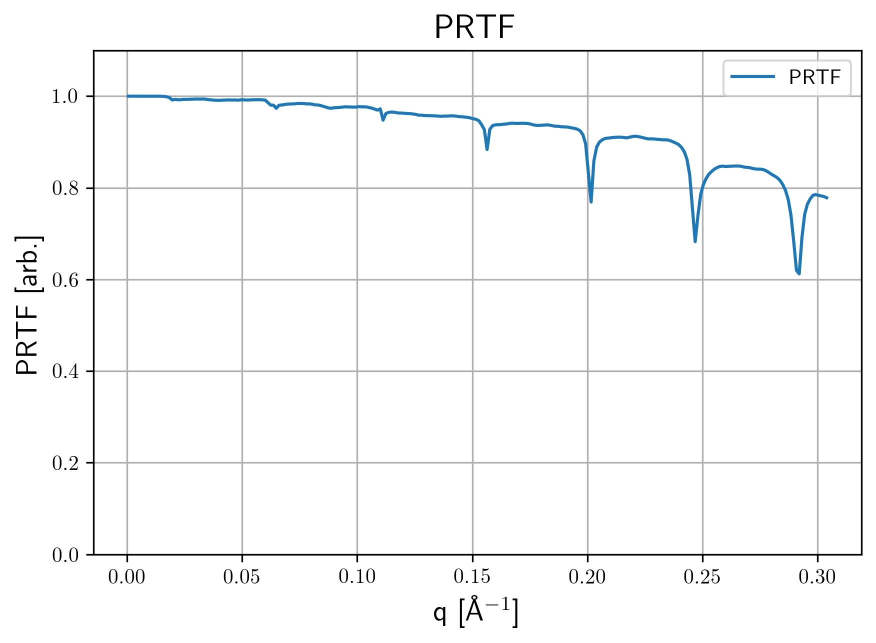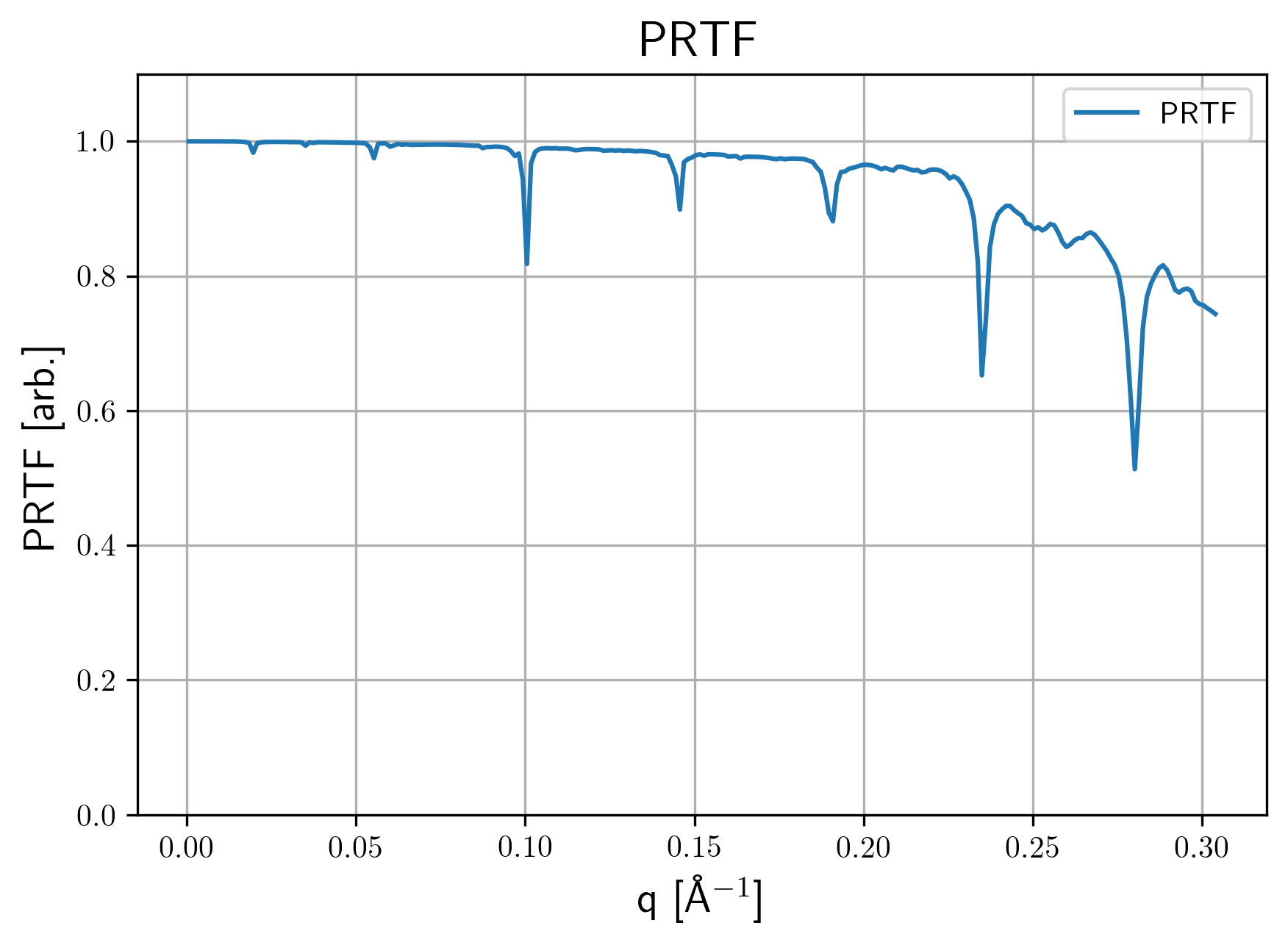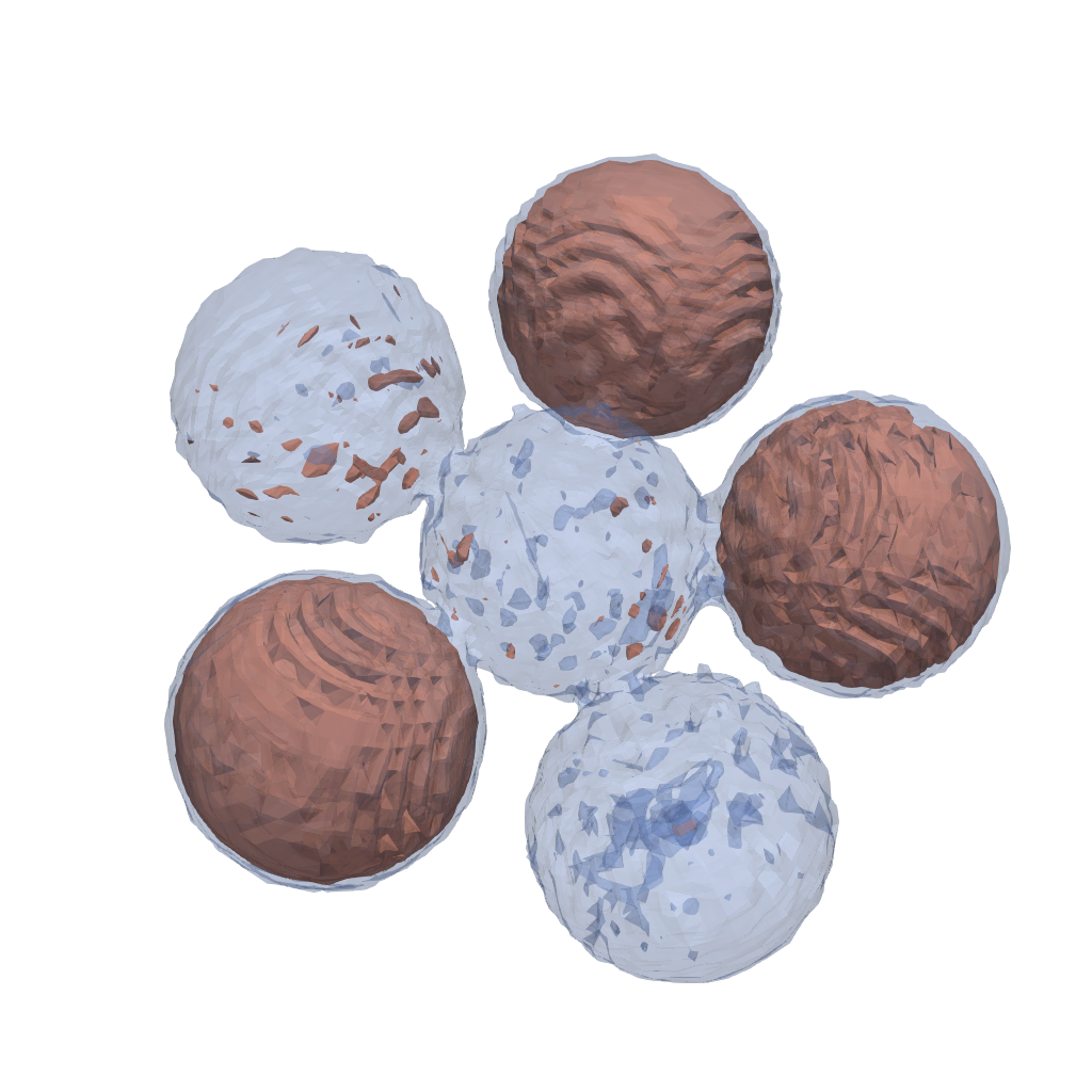
vtk Folder for vtk data files. Averaged reconstructions may look as follows

3d 1a.	3d 1b.	2d 1b.

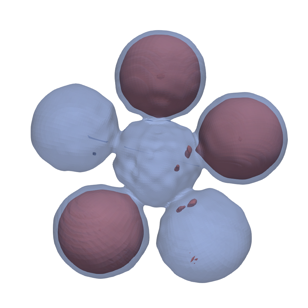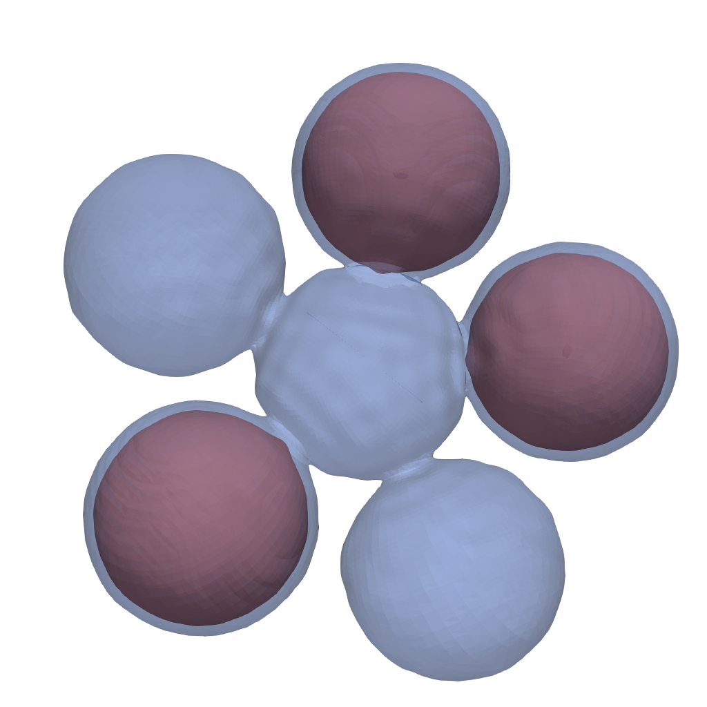average_results.h5 Main data output file.

average_results.h5 structure

average_results.h5
├aligned
│ └0
│   ├real_density 
│   └reciprocal_density 
├average
│ ├intensity_from_densities 
│ ├intensity_from_ft_densities
│ ├normalized_real_density
│ ├real_density
│ └reciprocal_density
├average_ids (1 attributes)
│ ├0
│ └1
├centered_average
│ ├normalized_real_density
│ ├real_density
│ └reciprocal_density
├input
│ ├0
│ │ ├real_density
│ │ ├reciprocal_density
│ │ └support_mask
│ └1
│   ├real_density
│   ├reciprocal_density
│   └support_mask
├input_meta
│ ├average_scaling_factors_per_file
│ ├grids
│ │ ├real_grid
│ │ └reciprocal_grid
│ ├projection_matrices (1 attributes)